Skills: A* algorithm, RRT, Graph-based search, path tracking, PID controller, differential drive robot, navigational & motion planner
Demo
This project includes the implementation of an A* search algorithm, and a Rapidly-Exploring Random Tree (RRT).
A* search algorithm:

Rapidly-Exploring Random Tree (RRT):
Contents
A* Search and Navigation
Overview
This project includes the implementation of an A* variant, able to generate 2D paths that navigate between the start and goal locations while avoiding obstacles, and a controller that enables a wheeled mobile robot to drive the generated paths.
Environment
- Landmarks from
MRCLAM_Dataset9, Robot3(Autonomous Space Robotics Lab, University of Toronto) (Link) was used as obstacles. - The robot is only able to observe the obstacles in its eight neighbor cells.
- Allowed cell transitions are its eight neighbor cells.
- True cost: +1 to move into an unoccupied neighbor cell, +1000 to move into a neighbor cell that is occupied.
Implementation
Heuristic function
The straight-line distance is calculated by:
$h = scale \times (x - x_G)^2 + (y - y_g)^2$
, Where x, y represents the current position and $x_G$, $y_G$ represents the goal position. Because the true cost of the robot moving diagonally is one and the straight-line distance would be $\sqrt 2$, the scale parameter is needed. Otherwise, the heuristic function may overestimate the true cost in this case.
Therefore, the path expansion is based on:
$f(n) = g(n) + h(n)$
, Where g denotes the true cost and h denoted the heuristic function.
Path planning
The visual display of the planned path is shown in the figure below. Blue cells are the occupied cells, and yellow cells are the planned path.

Online A*
The A* searching algorithm was then modified to be ‘online’. The difference between online and offline is that, when searching offline, the robot begins the movement after the expansion is completed. As the robot knows the obstacles in ‘offline’ searching, the algorithms can expand entirely before it starts to move the robot. The open list has cells that are not just their immediate neighbors. When the robot begins the movement, it only chooses the optimal path find by the algorithms. In the ‘online’ search, however, the robot may need to travel back and forth to find the best path when a new obstacle was detected.
I gave my ‘online’ searching robot the capability to memorize the position of the obstacles it has found. In other words, the robot is building a map while exploring the world. It may increase the computational load but would possibly find the path quicker when traveling to some area it has visited before.
The implementation of the ‘online’ searching version is based on the ‘offline’ version. The steps are summarized below:
- At the very beginning, the robot’s memory of the obstacles’ positions is an empty array. In other words, it does not have any prior knowledge of the world.
- The robot then looks at its eight immediate neighbors and add the obstacles to its memory (map) if there is any.
- The robot completes an A* star search based on this current memory (with knowledge on the current immediate neighbors and an empty array elsewhere) and finds a path. Since the robot does not know the obstacles that are not in its immediate neighbors, the planned path would just be a direct path to the goal.
- After that, the robot moves to the position next to its current location on the planned path, then looks at its new neighbors, add them to the memory, and re-plans with A* searching algorithms.
- The robot would repeat this ‘search, look, plan, move’ cycle until it moves to the goal.
Obstacle avoidance
The physical size of the robot is taken into account by inflating the obstacles. Squares approximate the inflated obstacles. The inflation method is shown in the figure below. Each obstacle was inflated by 0.3m in each direction. The corresponding cells were calculated. After that, all the 49 cells, as shown in the figure below, are labels as occupied.

The figure below is the visual display of the results (‘online’ searching) with 0.1 m grid size and inflated obstacles. As pointed out by the red arrow in the figure, the ‘online’ algorithm commands the robot to move left to move directly to the goal. Only when the obstacles are within the immediate neighbors of the robot, it decides to drive down to go around the occupied cells.

Controller
The controller is achieved by a proportional steering control and proportional speed control. For speed control, the velocity of the robot is proportional to the distance between the current position of the robot and the goal. To make the controller more realistic, the linear and angular acceleration was restricted within 0.288 m/s2 and 5.579 rad/s2, respectively.
The proportional gain for the linear and angular velocity was chosen to be 0.5 and 4, respectively. The final results are shown in Figure a below. Figure b shows the results without acceleration restrictions. Figures c and d show the movement of the robot with a smaller proportional gain and a larger proportional gain, respectively. When the gain is too small, the robot travels around with a large offset, which may cause the robot to move to its neighbor cell during the movement. A larger gain causes oscillation during the movement, as shown in Figure d.

Waypoints tracking
The figure below shows the robot tracking the waypoints (path) generated. Yellow cells are the planned path, and red arrows show the actual robot trajectory. The robot can move smoothly along the path.

To make the waypoint tracking more realistic, the noise was added to the motion model. The figure below illustrates the ‘driving while planning’ results. The algorithm was implemented with several modifications compared to the previous version.
- After each step of planning, the robot starts to execute the motion with the proportional controller from its current position to the next target node.
- If the robot successfully reached the goal, the searching algorithm begins to plan the next step.
- If the robot moves to an unintentional node instead of the target node, the robot will re-plan using its current position and the goal position.
- The current node, which the robot was unintentionally moved into, was added to the path. The targeted node, which the robot fails to reach, was deleted from the path.
- After re-planning, the robot controller moves the robot towards the next node.

‘Driving while planning’ results with a coarse grid are shown in the figure below.
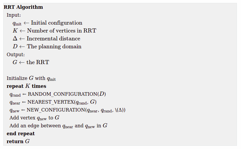
RRT Algorithm
Demo
Overview
This part of the project includes the implementation of Rapidly-Exploring Random Tree (RRT), a fundamental path planning algorithm.
The pseudocode for the algorithm is as follows:
Modules
simplerrt.py
A simple RRT algorithm in 2-D with the domain of [0,100]$\times$[0,100] and incremental distance as 1.
The figure below shows the algorithm after 500 and 5000 iterations. The RRT expanded in the free space with pretty uniform coverage over the whole space after 5000 iterations.


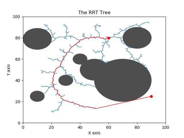
obstaclerrt.py
Circular obstacles are added to the domain. Collision checking is added to the algorithm.
The algorithm would terminate when it reached the goal and plot the path.
The plot below shows two trails with the same initial and goal position.
